Human Activity Detection using UCI’s HAR Dataset

IMU

Gait

Human Activity

Machine Learning

CNN

Classifying Accelerometer data to various activities of daily living (ADL) using Deep Learning.

Published

September 25, 2025

Okay, now we are stepping things up a little bit. This time, the data comes from UCI. According to the website:

For each record in the dataset it is provided: - Triaxial acceleration from the accelerometer (total acceleration) and the estimated body acceleration. - Triaxial Angular velocity from the gyroscope. - A 561-feature vector with time and frequency domain variables. - Its activity label. - An identifier of the subject who carried out the experiment.

The dataset is a bit different - it’s already been divided into train and test sets but they are all text files. Once again, let’s get into it - for fun, let’s also use the same model from last time to see if that architecture still works fine for this dataset. If it doesn’t, let’s see if we can build a different one.

Load Data

The data is split into total, body and gyro - these are the sensor values. There’s also another dataset that has some 561 features extracted from this. Might be fun to play with them but for now, let’s focus on building our CNN network - so this ‘total’ values would be fine for now. May play with .body’ accel values later.

file_location = '/Users/manikandanravi/Code/quarto-test/uci-har-dataset/train/Inertial Signals/total_acc_x_train.txt' # Update this path to your file location

# Load into pandas
import pandas as pd
import re

data = pd.read_csv(file_location, sep='\s+', header=None)
display(data.head())
data.shape

<>:7: SyntaxWarning: invalid escape sequence '\s'
<>:7: SyntaxWarning: invalid escape sequence '\s'
/var/folders/q7/ftl_yg4n1gndbwlnk654hq1h0000gn/T/ipykernel_99227/3576027909.py:7: SyntaxWarning: invalid escape sequence '\s'
  data = pd.read_csv(file_location, sep='\s+', header=None)

	0	1	2	3	4	5	6	7	8	9	...	118	119	120	121	122	123	124	125	126	127
0	1.012817	1.022833	1.022028	1.017877	1.023680	1.016974	1.017746	1.019263	1.016417	1.020745	...	1.020981	1.018065	1.019638	1.020017	1.018766	1.019815	1.019290	1.018445	1.019372	1.021171
1	1.018851	1.022380	1.020781	1.020218	1.021344	1.020522	1.019790	1.019216	1.018307	1.017996	...	1.019291	1.019258	1.020736	1.020950	1.020491	1.018685	1.015660	1.014788	1.016499	1.017849
2	1.023127	1.021882	1.019178	1.015861	1.012893	1.016451	1.020331	1.020266	1.021759	1.018649	...	1.020304	1.021516	1.019417	1.019312	1.019448	1.019434	1.019916	1.021041	1.022935	1.022019
3	1.017682	1.018149	1.019854	1.019880	1.019121	1.020479	1.020595	1.016340	1.010611	1.009013	...	1.021295	1.022934	1.022183	1.021637	1.020598	1.018887	1.019161	1.019916	1.019602	1.020735
4	1.019952	1.019616	1.020933	1.023061	1.022242	1.020867	1.021939	1.022300	1.022302	1.022254	...	1.022687	1.023670	1.019899	1.017381	1.020389	1.023884	1.021753	1.019425	1.018896	1.016787

5 rows × 128 columns

(7352, 128)

# Let's see how the labels look like

file_location = '/Users/manikandanravi/Code/quarto-test/uci-har-dataset/train/y_train.txt'

# Load
data = pd.read_csv(file_location, sep='\s+', header=None)
display(data.head())
data.shape

<>:6: SyntaxWarning: invalid escape sequence '\s'
<>:6: SyntaxWarning: invalid escape sequence '\s'
/var/folders/q7/ftl_yg4n1gndbwlnk654hq1h0000gn/T/ipykernel_99227/3965665900.py:6: SyntaxWarning: invalid escape sequence '\s'
  data = pd.read_csv(file_location, sep='\s+', header=None)

	0
0	5
1	5
2	5
3	5
4	5

(7352, 1)

Okay looks like there are 7352 segments of windowed data with associated labels

Make a Dataframe

# Load X axis data
file_location = '/Users/manikandanravi/Code/quarto-test/uci-har-dataset/train/Inertial Signals/total_acc_x_train.txt'
df_total = pd.read_csv(file_location, sep='\s+', header=None)
file_loc_body = '/Users/manikandanravi/Code/quarto-test/uci-har-dataset/train/Inertial Signals/body_acc_x_train.txt'
df_body = pd.read_csv(file_loc_body, sep='\s+', header=None)
file_loc_gyro = '/Users/manikandanravi/Code/quarto-test/uci-har-dataset/train/Inertial Signals/body_gyro_x_train.txt'
df_gyro = pd.read_csv(file_loc_gyro, sep='\s+', header=None)

# Append Y axis data
file_location = '/Users/manikandanravi/Code/quarto-test/uci-har-dataset/train/Inertial Signals/total_acc_y_train.txt'
df_total = pd.concat([df_total, pd.read_csv(file_location, sep='\s+', header=None)], axis=1)
file_loc_body = '/Users/manikandanravi/Code/quarto-test/uci-har-dataset/train/Inertial Signals/body_acc_y_train.txt'
df_body = pd.concat([df_body, pd.read_csv(file_loc_body, sep='\s+', header=None)], axis=1)
file_loc_gyro = '/Users/manikandanravi/Code/quarto-test/uci-har-dataset/train/Inertial Signals/body_gyro_y_train.txt'
df_gyro = pd.concat([df_gyro, pd.read_csv(file_loc_gyro, sep='\s+', header=None)], axis=1)

# Z axis
file_location = '/Users/manikandanravi/Code/quarto-test/uci-har-dataset/train/Inertial Signals/total_acc_z_train.txt'
df_total = pd.concat([df_total, pd.read_csv(file_location, sep='\s+', header=None)], axis=1)
file_loc_body = '/Users/manikandanravi/Code/quarto-test/uci-har-dataset/train/Inertial Signals/body_acc_z_train.txt'
df_body = pd.concat([df_body, pd.read_csv(file_loc_body, sep='\s+', header=None)], axis=1)
file_loc_gyro = '/Users/manikandanravi/Code/quarto-test/uci-har-dataset/train/Inertial Signals/body_gyro_z_train.txt'
df_gyro = pd.concat([df_gyro, pd.read_csv(file_loc_gyro, sep='\s+', header=None)], axis=1)

# Labels
file_location = '/Users/manikandanravi/Code/quarto-test/uci-har-dataset/train/y_train.txt'
y_train = pd.read_csv(file_location, sep='\s+', header=None)
# Subtract 1 from values
y_train -= 1

df_total.shape, df_body.shape, y_train.shape

((7352, 384), (7352, 384), (7352, 1))

# Load into 3 dimensional numpy arrays

import numpy as np

X_total_train = df_total.values.reshape(7352, 128, 3)
X_body_train = df_body.values.reshape(7352, 128, 3)
X_gyro_train = df_gyro.values.reshape(7352, 128, 3)
y_train = np.array(y_train)

# Do the same for test data

# Load X axis data
file_location = '/Users/manikandanravi/Code/quarto-test/uci-har-dataset/test/Inertial Signals/total_acc_x_test.txt'
df_total_test = pd.read_csv(file_location, sep='\s+', header=None)
file_loc_body = '/Users/manikandanravi/Code/quarto-test/uci-har-dataset/test/Inertial Signals/body_acc_x_test.txt'
df_body_test = pd.read_csv(file_loc_body, sep='\s+', header=None)
file_loc_gyro = '/Users/manikandanravi/Code/quarto-test/uci-har-dataset/test/Inertial Signals/body_gyro_x_test.txt'
df_gyro = pd.read_csv(file_loc_gyro, sep='\s+', header=None)

# Append Y axis data
file_location = '/Users/manikandanravi/Code/quarto-test/uci-har-dataset/test/Inertial Signals/total_acc_y_test.txt'
df_total_test = pd.concat([df_total_test, pd.read_csv(file_location, sep='\s+', header=None)], axis=1)
file_loc_body = '/Users/manikandanravi/Code/quarto-test/uci-har-dataset/test/Inertial Signals/body_acc_y_test.txt'
df_body_test = pd.concat([df_body_test, pd.read_csv(file_loc_body, sep='\s+', header=None)], axis=1)
file_loc_gyro = '/Users/manikandanravi/Code/quarto-test/uci-har-dataset/test/Inertial Signals/body_gyro_y_test.txt'
df_gyro = pd.concat([df_gyro, pd.read_csv(file_loc_gyro, sep='\s+', header=None)], axis=1)

# Z axis
file_location = '/Users/manikandanravi/Code/quarto-test/uci-har-dataset/test/Inertial Signals/total_acc_z_test.txt'
df_total_test = pd.concat([df_total_test, pd.read_csv(file_location, sep='\s+', header=None)], axis=1)
file_loc_body = '/Users/manikandanravi/Code/quarto-test/uci-har-dataset/test/Inertial Signals/body_acc_z_test.txt'
df_body_test = pd.concat([df_body_test, pd.read_csv(file_loc_body, sep='\s+', header=None)], axis=1)
file_loc_gyro = '/Users/manikandanravi/Code/quarto-test/uci-har-dataset/test/Inertial Signals/body_gyro_z_test.txt'
df_gyro = pd.concat([df_gyro, pd.read_csv(file_loc_gyro, sep='\s+', header=None)], axis=1)

# Labels
file_location = '/Users/manikandanravi/Code/quarto-test/uci-har-dataset/test/y_test.txt'
y_test = pd.read_csv(file_location, sep='\s+', header=None)
y_test -= 1

# Convert to numpy arrays
X_total_test = df_total_test.values.reshape(len(df_total_test), 128, 3)
X_body_test = df_body_test.values.reshape(len(df_body_test), 128, 3)
X_gyro_test = df_gyro.values.reshape(len(df_gyro), 128, 3)
y_test = np.array(y_test)

print("Shapes of test data:")
print("X_total_test:", X_total_test.shape)
print("X_body_test:", X_body_test.shape)
print("X_gyro_test:", X_gyro_test.shape)
print("y_test:", y_test.shape)

OKay, now we have the data. Let’s get to work on building dataloaders and the models

Build Model

Data Loader

import torch
import torch.nn as nn
from torch.utils.data import Dataset, DataLoader

# Dataset wrapper
class UCIDatasetWrapper(Dataset):
  def __init__(self, X, y):
    # Convert (N, T, C) -> (N, C, T) for Conv1D
    self.X = torch.tensor(X.transpose(0,2,1), dtype=torch.float32)
    self.y = torch.tensor(y, dtype=torch.long)

  def __len__(self):
    return len(self.y)

  def __getitem__(self, i):
    return self.X[i], self.y[i]

  train_ds = UCIDatasetWrapper(X_total_train, y_train)
  train_ds_body = UCIDatasetWrapper(X_body_train, y_train)
  test_ds = UCIDatasetWrapper(X_total_test, y_test)
  test_ds_body = UCIDatasetWrapper(X_body_test, y_test)

  train_dl = DataLoader(train_ds, batch_size=32, shuffle=True)
  train_dl_body = DataLoader(train_ds_body, batch_size=32, shuffle=True)
  test_dl = DataLoader(test_ds, batch_size=32, shuffle=False)

Model

Lets use the same model from the previous notbook

# 1D CNN model (Same as our previous notebook)
import torch.nn.functional as F
class HAR1DCNN(nn.Module):
    def __init__(self, in_channels=3, n_classes=6):  # adjust n_classes!
        super().__init__()
        self.conv1 = nn.Conv1d(in_channels, 32, kernel_size=3, padding=1)
        self.bn1 = nn.BatchNorm1d(32)
        self.conv2 = nn.Conv1d(32, 64, kernel_size=3, padding=1)
        self.bn2 = nn.BatchNorm1d(64)
        self.pool = nn.MaxPool1d(2)
        self.conv3 = nn.Conv1d(64, 128, kernel_size=3, padding=1)
        self.bn3 = nn.BatchNorm1d(128)
        self.global_pool = nn.AdaptiveAvgPool1d(1)
        self.fc = nn.Linear(128, n_classes)

    def forward(self, x):
        x = F.relu(self.bn1(self.conv1(x)))
        x = self.pool(x)          # (N, 32, 20)
        x = F.relu(self.bn2(self.conv2(x)))
        x = self.pool(x)          # (N, 64, 10)
        x = F.relu(self.bn3(self.conv3(x)))
        x = self.global_pool(x).squeeze(-1)  # (N, 128)
        return self.fc(x)

Train the model

device = torch.device("cuda" if torch.cuda.is_available() else "cpu")
if device.type != "cuda":
  device = torch.device("mps" if torch.backends.mps.is_available() else "cpu")

n_classes = len(torch.unique(torch.tensor(y_train)))
model = HAR1DCNN(in_channels=3, n_classes=n_classes).to(device)

# Optimizer and loss function
optim = torch.optim.Adam(model.parameters(), lr=1e-3)
loss_fn = nn.CrossEntropyLoss()

def run_epoch(loader, train=True):
  if train:
    model.train()
  else:
    model.eval()
  total_loss, correct, total = 0, 0, 0
  for Xb, yb in loader:
    Xb, yb = Xb.to(device), yb.to(device)
    if train:
      optim.zero_grad()
    out = model(Xb)
    loss = loss_fn(out, yb.squeeze()) # Removed - 1
    if train:
      loss.backward()
      optim.step()

    total_loss += loss.item() * Xb.size(0)
    preds = out.argmax(1)

    correct += (preds == yb.squeeze()).sum().item() # Removed - 1
    total += Xb.size(0)
  return total_loss/total, correct/total

for epoch in range(10):
  train_loss, train_acc = run_epoch(train_dl)
  test_loss, test_acc = run_epoch(test_dl, train=False)
  print(f'Epoch {epoch+1}: train_loss={train_loss:.4f}, train_acc={train_acc:.4f}, test_loss={test_loss:.4f}, test_acc={test_acc:.4f}')

Epoch 1: train_loss=0.6116, train_acc=0.8156, test_loss=0.4655, test_acc=0.7815
Epoch 2: train_loss=0.2725, train_acc=0.9063, test_loss=0.5308, test_acc=0.7815
Epoch 3: train_loss=0.2072, train_acc=0.9237, test_loss=0.2954, test_acc=0.8839
Epoch 4: train_loss=0.1807, train_acc=0.9295, test_loss=0.2947, test_acc=0.8775
Epoch 5: train_loss=0.1657, train_acc=0.9342, test_loss=0.3485, test_acc=0.8772
Epoch 6: train_loss=0.1620, train_acc=0.9353, test_loss=0.2724, test_acc=0.9118
Epoch 7: train_loss=0.1496, train_acc=0.9373, test_loss=0.2644, test_acc=0.8972
Epoch 8: train_loss=0.1495, train_acc=0.9373, test_loss=0.4436, test_acc=0.8314
Epoch 9: train_loss=0.1502, train_acc=0.9399, test_loss=0.4513, test_acc=0.8354
Epoch 10: train_loss=0.1378, train_acc=0.9433, test_loss=0.2238, test_acc=0.9199

Evaluate model

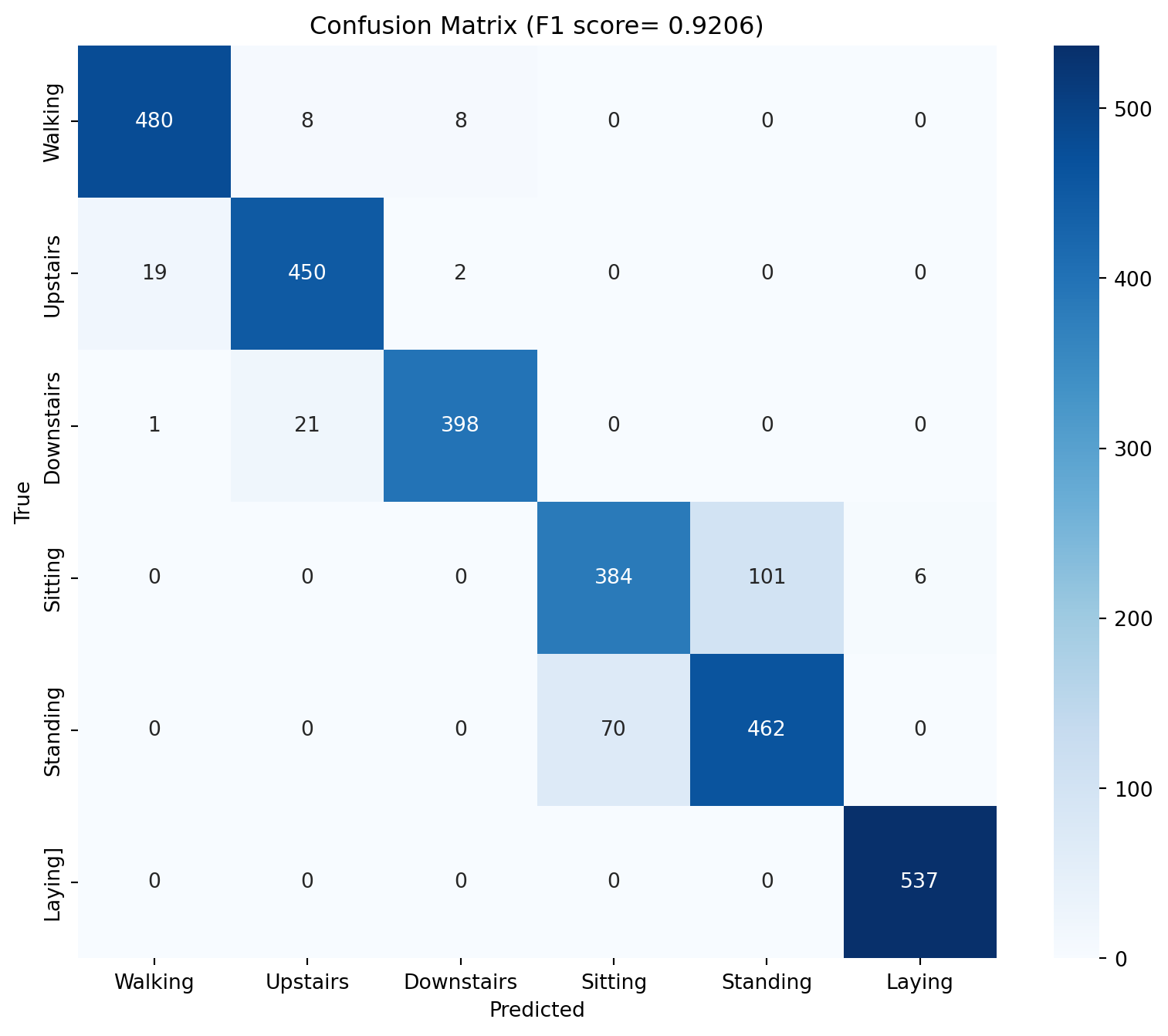
# Evaluate the model - get F1 score, confusion matrix

from sklearn.metrics import f1_score, confusion_matrix

model.eval()
y_pred = []
y_true = []
with torch.no_grad():
    for Xb, yb in test_dl:
        Xb, yb = Xb.to(device), yb.to(device)
        out = model(Xb)
        preds = out.argmax(1)
        y_pred.extend(preds.cpu().numpy())
        y_true.extend(yb.cpu().numpy())

f1 = f1_score(y_true, y_pred, average='macro')
cm = confusion_matrix(y_true, y_pred)
print(f'F1 score: {f1:.4f}')

# PLot confusion matrix

import seaborn as sns
import matplotlib.pyplot as plt

plt.figure(figsize=(10, 8))
sns.heatmap(cm, annot=True, fmt='d', cmap='Blues')
plt.xlabel('Predicted')
plt.ylabel('True')
plt.title(f'Confusion Matrix (F1 score= {f1:.4f})')
plt.xticks([0.5, 1.5, 2.5, 3.5, 4.5, 5.5], ['Walking', 'Upstairs', 'Downstairs', 'Sitting', 'Standing', 'Laying'])
plt.yticks([0.5, 1.5, 2.5, 3.5, 4.5, 5.5], ['Walking', 'Upstairs', 'Downstairs', 'Sitting', 'Standing', 'Laying]'])
plt.show()

F1 score: 0.9206

Changing Data

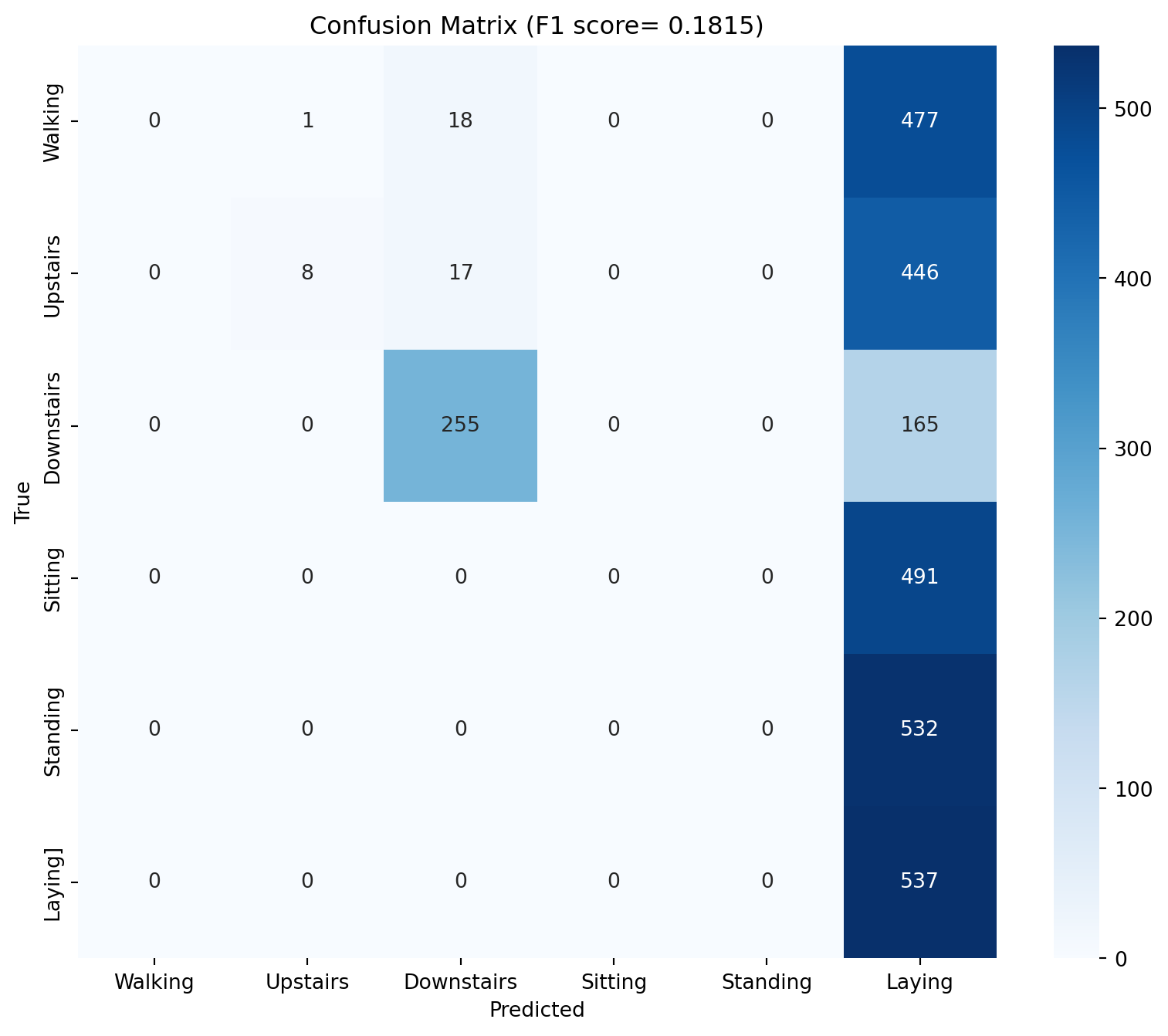
What if we train the model just with the ‘body’ accelerometer data?

Just to recap: > The sensor signals (accelerometer and gyroscope) were pre-processed by applying noise filters and then sampled in fixed-width sliding windows of 2.56 sec and 50% overlap (128 readings/window). The sensor acceleration signal, which has gravitational and body motion components, was separated using a Butterworth low-pass filter into body acceleration and gravity. The gravitational force is assumed to have only low frequency components, therefore a filter with 0.3 Hz cutoff frequency was used. From each window, a vector of features was obtained by calculating variables from the time and frequency domain.

for epoch in range(10):
  train_loss, train_acc = run_epoch(train_dl_body)
  test_loss, test_acc = run_epoch(test_dl, train=False)
  print(f'Epoch {epoch+1}: train_loss={train_loss:.4f}, train_acc={train_acc:.4f}, test_loss={test_loss:.4f}, test_acc={test_acc:.4f}')

Epoch 1: train_loss=0.7446, train_acc=0.5947, test_loss=4.3886, test_acc=0.4055
Epoch 2: train_loss=0.6669, train_acc=0.6287, test_loss=5.8494, test_acc=0.3590
Epoch 3: train_loss=0.6581, train_acc=0.6363, test_loss=10.5056, test_acc=0.3156
Epoch 4: train_loss=0.6429, train_acc=0.6341, test_loss=8.6658, test_acc=0.3146
Epoch 5: train_loss=0.6239, train_acc=0.6391, test_loss=7.5618, test_acc=0.2820
Epoch 6: train_loss=0.6272, train_acc=0.6431, test_loss=12.1228, test_acc=0.2633
Epoch 7: train_loss=0.6199, train_acc=0.6440, test_loss=9.1903, test_acc=0.2803
Epoch 8: train_loss=0.6179, train_acc=0.6578, test_loss=16.8655, test_acc=0.2847
Epoch 9: train_loss=0.6167, train_acc=0.6533, test_loss=14.1179, test_acc=0.3010
Epoch 10: train_loss=0.6167, train_acc=0.6570, test_loss=16.3485, test_acc=0.2715

# Evaluate the model - get F1 score, confusion matrix

from sklearn.metrics import f1_score, confusion_matrix

model.eval()
y_pred = []
y_true = []
with torch.no_grad():
    for Xb, yb in test_dl:
        Xb, yb = Xb.to(device), yb.to(device)
        out = model(Xb)
        preds = out.argmax(1)
        y_pred.extend(preds.cpu().numpy())
        y_true.extend(yb.cpu().numpy())

f1 = f1_score(y_true, y_pred, average='macro')
cm = confusion_matrix(y_true, y_pred)
print(f'F1 score: {f1:.4f}')

# PLot confusion matrix

import seaborn as sns
import matplotlib.pyplot as plt

plt.figure(figsize=(10, 8))
sns.heatmap(cm, annot=True, fmt='d', cmap='Blues')
plt.xlabel('Predicted')
plt.ylabel('True')
plt.title(f'Confusion Matrix (F1 score= {f1:.4f})')
plt.xticks([0.5, 1.5, 2.5, 3.5, 4.5, 5.5], ['Walking', 'Upstairs', 'Downstairs', 'Sitting', 'Standing', 'Laying'])
plt.yticks([0.5, 1.5, 2.5, 3.5, 4.5, 5.5], ['Walking', 'Upstairs', 'Downstairs', 'Sitting', 'Standing', 'Laying]'])
plt.show()

F1 score: 0.1815

As we can see (and intutitively expect), if we take out the gravitational component, the accuracy values are pretty poor. What if we feed all these 9 vectors in?

Running the model with all the data

# Concatenate total, body and gyro

X_all_train = np.concat((X_total_train, X_body_train, X_gyro_train), axis=2)
display(X_all_train.shape, y_train.shape) # We should have 9 channels now
X_all_test = np.concat((X_total_test, X_body_test, X_gyro_test), axis=2)
display(X_all_test.shape, y_test.shape)

(7352, 128, 9)

(7352, 1)

(2947, 128, 9)

(2947, 1)

# Create data loaders

train_ds_all = UCIDatasetWrapper(X_all_train, y_train)
train_dl_all = DataLoader(train_ds_all, batch_size=32, shuffle=True)
test_ds_all = UCIDatasetWrapper(X_all_test, y_test)
test_dl_all = DataLoader(test_ds_all, batch_size=32, shuffle=False)

# We need a new model with 9 channels

class HAR1DCNN_9ch(nn.Module):
    def __init__(self, in_channels=9, n_classes=6):  # adjust n_classes!
        super().__init__()
        self.conv1 = nn.Conv1d(in_channels, 32, kernel_size=3, padding=1)
        self.bn1 = nn.BatchNorm1d(32)
        self.conv2 = nn.Conv1d(32, 64, kernel_size=3, padding=1)
        self.bn2 = nn.BatchNorm1d(64)
        self.pool = nn.MaxPool1d(2)
        self.conv3 = nn.Conv1d(64, 128, kernel_size=3, padding=1)
        self.bn3 = nn.BatchNorm1d(128)
        self.global_pool = nn.AdaptiveAvgPool1d(1)
        self.fc = nn.Linear(128, n_classes)

    def forward(self, x):
        x = F.relu(self.bn1(self.conv1(x)))
        x = self.pool(x)          # (N, 32, 20)
        x = F.relu(self.bn2(self.conv2(x)))
        x = self.pool(x)          # (N, 64, 10)
        x = F.relu(self.bn3(self.conv3(x)))
        x = self.global_pool(x).squeeze(-1)  # (N, 128)
        return self.fc(x)

Train the new model

device = torch.device("cuda" if torch.cuda.is_available() else "cpu")
if device.type != "cuda":
  device = torch.device("mps" if torch.backends.mps.is_available() else "cpu")
n_classes = len(torch.unique(torch.tensor(y_train)))
model_2 = HAR1DCNN_9ch(in_channels=9, n_classes=n_classes).to(device)

# Optimizer and loss function
optim = torch.optim.Adam(model_2.parameters(), lr=1e-3)
loss_fn = nn.CrossEntropyLoss()

def run_epoch(loader, train=True):
  if train:
    model_2.train()
  else:
    model_2.eval()
  total_loss, correct, total = 0, 0, 0
  for Xb, yb in loader:
    Xb, yb = Xb.to(device), yb.to(device)
    if train:
      optim.zero_grad()
    out = model_2(Xb)
    loss = loss_fn(out, yb.squeeze())
    if train:
      loss.backward()
      optim.step()

    total_loss += loss.item() * Xb.size(0)
    preds = out.argmax(1)

    correct += (preds == yb.squeeze()).sum().item()
    total += Xb.size(0)
  return total_loss/total, correct/total

for epoch in range(20):
  train_loss, train_acc = run_epoch(train_dl_all)
  test_loss, test_acc = run_epoch(test_dl_all, train=False)
  print(f'Epoch {epoch+1}: train_loss={train_loss:.4f}, train_acc={train_acc:.4f}, test_loss={test_loss:.4f}, test_acc={test_acc:.4f}')

Epoch 1: train_loss=0.5799, train_acc=0.8203, test_loss=0.3687, test_acc=0.8748
Epoch 2: train_loss=0.2129, train_acc=0.9267, test_loss=0.3317, test_acc=0.8622
Epoch 3: train_loss=0.1801, train_acc=0.9317, test_loss=0.3841, test_acc=0.8571
Epoch 4: train_loss=0.1486, train_acc=0.9388, test_loss=0.2287, test_acc=0.9169
Epoch 5: train_loss=0.1417, train_acc=0.9382, test_loss=0.2518, test_acc=0.9080
Epoch 6: train_loss=0.1381, train_acc=0.9421, test_loss=0.2403, test_acc=0.9192
Epoch 7: train_loss=0.1242, train_acc=0.9509, test_loss=0.2335, test_acc=0.9203
Epoch 8: train_loss=0.1198, train_acc=0.9490, test_loss=0.2324, test_acc=0.9311
Epoch 9: train_loss=0.1206, train_acc=0.9484, test_loss=0.2452, test_acc=0.9148
Epoch 10: train_loss=0.1190, train_acc=0.9497, test_loss=0.2798, test_acc=0.9016
Epoch 11: train_loss=0.1078, train_acc=0.9561, test_loss=0.2884, test_acc=0.9077
Epoch 12: train_loss=0.1212, train_acc=0.9483, test_loss=0.2468, test_acc=0.9230
Epoch 13: train_loss=0.1124, train_acc=0.9529, test_loss=0.2659, test_acc=0.9125
Epoch 14: train_loss=0.1144, train_acc=0.9544, test_loss=0.2195, test_acc=0.9379
Epoch 15: train_loss=0.1063, train_acc=0.9563, test_loss=0.2379, test_acc=0.9304
Epoch 16: train_loss=0.1037, train_acc=0.9591, test_loss=0.3022, test_acc=0.9179
Epoch 17: train_loss=0.1060, train_acc=0.9573, test_loss=0.2041, test_acc=0.9362
Epoch 18: train_loss=0.1008, train_acc=0.9585, test_loss=0.2672, test_acc=0.9196
Epoch 19: train_loss=0.1024, train_acc=0.9581, test_loss=0.2157, test_acc=0.9389
Epoch 20: train_loss=0.1033, train_acc=0.9554, test_loss=0.3729, test_acc=0.8836

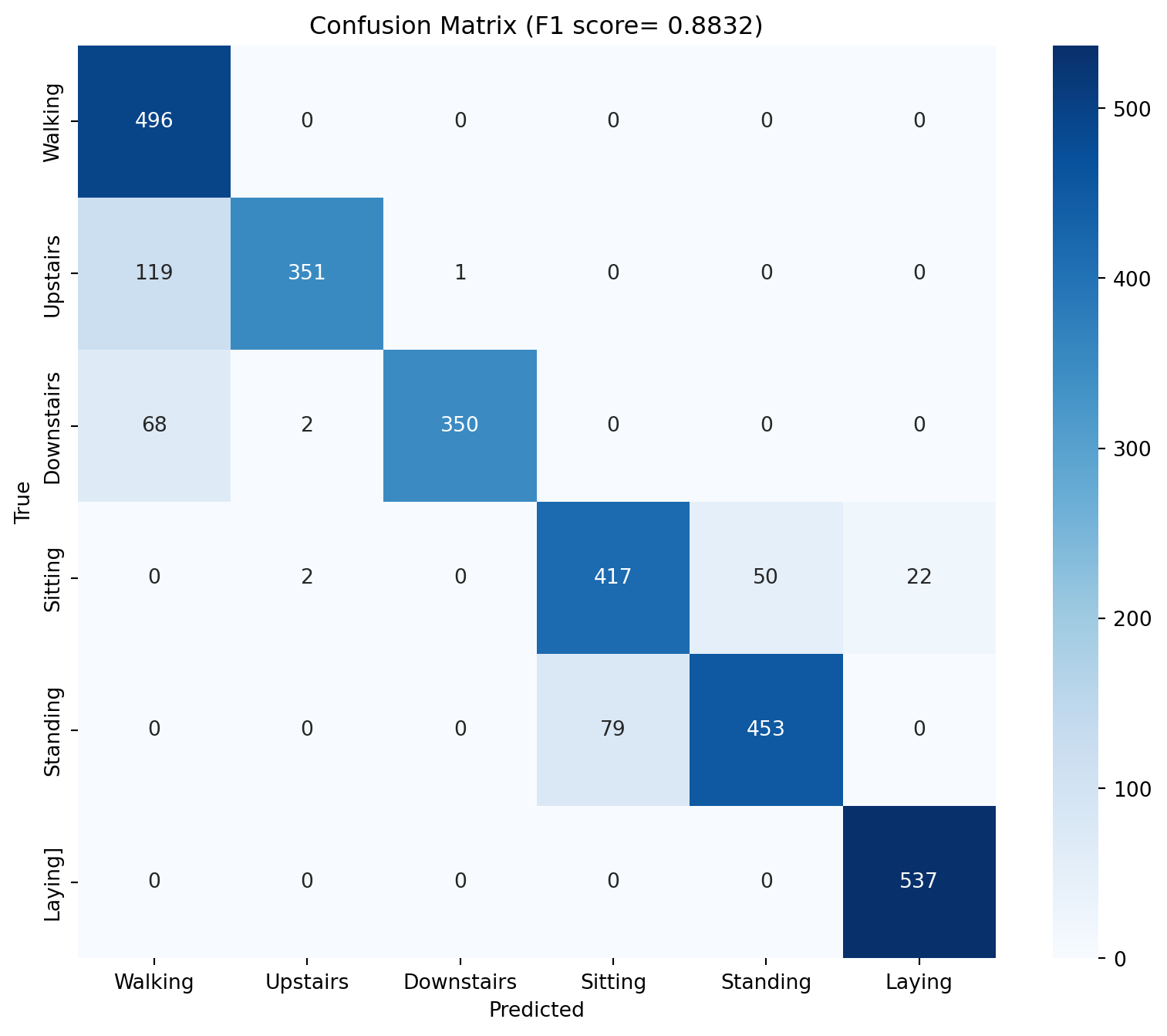
# Evaluate the model - get F1 score, confusion matrix

from sklearn.metrics import f1_score, confusion_matrix

model_2.eval()
y_pred = []
y_true = []
with torch.no_grad():
    for Xb, yb in test_dl_all:
        Xb, yb = Xb.to(device), yb.to(device)
        out = model_2(Xb)
        preds = out.argmax(1)
        y_pred.extend(preds.cpu().numpy())
        y_true.extend(yb.cpu().numpy())

f1 = f1_score(y_true, y_pred, average='macro')
cm = confusion_matrix(y_true, y_pred)
print(f'F1 score: {f1:.4f}')

# PLot confusion matrix

import seaborn as sns
import matplotlib.pyplot as plt

plt.figure(figsize=(10, 8))
sns.heatmap(cm, annot=True, fmt='d', cmap='Blues')
plt.xlabel('Predicted')
plt.ylabel('True')
plt.title(f'Confusion Matrix (F1 score= {f1:.4f})')
plt.xticks([0.5, 1.5, 2.5, 3.5, 4.5, 5.5], ['Walking', 'Upstairs', 'Downstairs', 'Sitting', 'Standing', 'Laying'])
plt.yticks([0.5, 1.5, 2.5, 3.5, 4.5, 5.5], ['Walking', 'Upstairs', 'Downstairs', 'Sitting', 'Standing', 'Laying]'])
plt.show()

F1 score: 0.8832

As we can see, this has improved on the accuracy on our first model (albeit, not by a lot - because our first model was already quite good).